The Problem
I’ve been working on a side project to log real-time traffic statistics across Singapore and make the historic data publicly available. The real time APIs from LTA refreshes data at 1-5 minute intervals. While I’m only querying the APIs once every 15 minutes, some of the data is really rich, and file sizes add up quickly. This accumulates as storage costs on Google Cloud Platform. In particular, the traffic-speed-bands API provides speed bands (10kmh ranges) of almost 60k road stretches across Singapore every 5 minutes.
First, I removed relatively constant fields and stored them as metadata. This was somewhat effective as many of the constant fields were road or place names, strings which took considerable space. However, that didn’t seem to be sufficient in my quest to keep costs for the project to a minimum. I was processing the data using Pandas, and as Pandas itself is able to handle compression, things were pretty convenient. I just had to figure out which compression mode to use.
Pandas Compression Modes
Pandas’ to_csv function supports a parameter compression. By default it takes the value 'infer', which infers the compression mode from the destination path provided. Alternatively, these are the supported options for compression:
'gzip''bz2''zip''xz'None
Likewise, read_csv supports the compression parameter, which it infers from the specified path by default, or accepts any of the above options. When reading a CSV file that has been compressed with any of the above formats, instead of needing to decompress the file before passing it through read_csv, the compresseed file can be passed directly through read_csv.
Next, finding out how much each compression mode saves on storage space, and the tradeoffs in speed.
The experiment
To compare the different compression formats, I first generated CSV files for the 6 datasets I was logging data for. Each dataset was different in terms of average size and the types of data stored. Some had purely floats, while some had a mix of strings and floats. Each run was saved to a CSV file. I ran these for 9 days, once every 15 minutes. These totaled to approximately 864 files per dataset (slightly less due to errors with some runs).
For some datasets, the number of rows are almost always the same in each query, as they come from specific meters/ measurement points along roads. Sizes for these files are very similar. Other APIs are not tagged to specific locations, such as availability of taxis or incidents reported. These datasets have no fixed number of rows and sizes vary widely.
Next, I opened the CSV files with Pandas as a dataframe and saved them with each of the compression formats. I compared the start and end sizes, as well as the write times. Noting that speed performance over time may vary, I shuffled the files before processing to ensure that such performance differences would not accumulate at any particular dataset or date range.
Finally, I opened each of the compressed files and compared the time required to load each of these files as a dataframe, also shuffling the files before running the tasks.
Here’s an interactive version of the charts below.
Comparison of Compression Rates
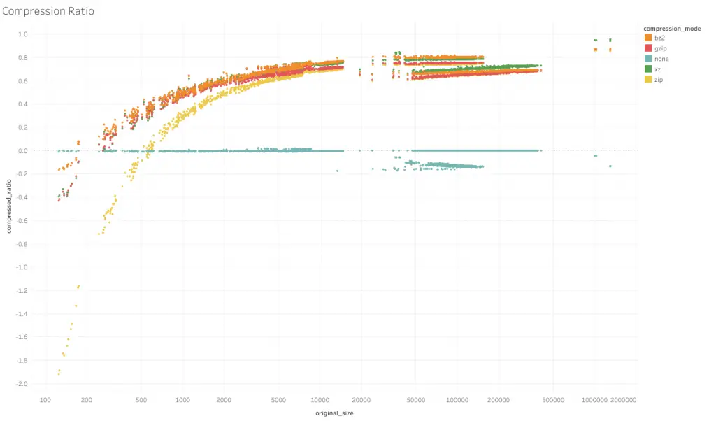
On the horizontal axis is the original file size in bytes, on a log scale. The compressed ratio, or 1- (size of compressed file divided by original size), is on the vertical axis. A higher number indicates that the output file size is smaller (as a ratio of the original). A number below 0 indicates the file got larger.
From the shape of the chart, it appears that larger file sizes benefit more from compression. On the far end this range size savings are over 90%. At smaller file sizes, compression may even make the file larger.
compression=None
For compression=None, the ratio hovers around 0, indicating not much changes to file size, as expected. However, around the middle portion there are a bunch of files which got larger after compression, which was interesting. It appears that most of these were from a dataset which consists of only floats (taxi-availability).
compression='zip'
Generally, compression='zip' (yellow line) performs worse than the other compression formats, though the difference narrows as file sizes got larger.
compression='gzip'
Compression ratios of the remaining 3 formats are much closer, though it seems that of the 3, compression='gzip' (red line) seems to have the lowest compression rates across the spectrum.
compression='bz2' and compression='xz'
Between compression='bz2' (orange) and compression='xz' (green), the results are slightly more interesting. Looking at the bunch of lines to the center-right, the higher 3 belong to one dataset (taxi-availability) and the lower 3 belong to another (traffic-images-detections). The group for taxi-availability is ordered orange-green-red (bz2–xz–gzip) from best to worst ratios, whereas for traffic-images-detections, xz outperforms bz2.
I’m not sure of the exact reasons but a point to note is that taxi-availability consists of only floats, while traffic-images-detections is a mix of strings and floats. It also appears that for the taxi-availability group, compression ratios are flat across the group. For the traffic-images-detections group, while having less compression than the taxi-availability group, experiences greater compression ratios as size gets larger. It appears that for pure floats, 'bz2' performs better while for a mix with strings, 'xz' does better.
At the far right of the chart are the largest files and where I’m most concerned about. These files, from the traffic-speed-bands API, consist of strings and integers, and 'xz' performs significantly better than the other compression modes. 'xz' format compresses to around 95% of the original size while 'bz2' compresses to about 87%.
Comparison of Write Speed
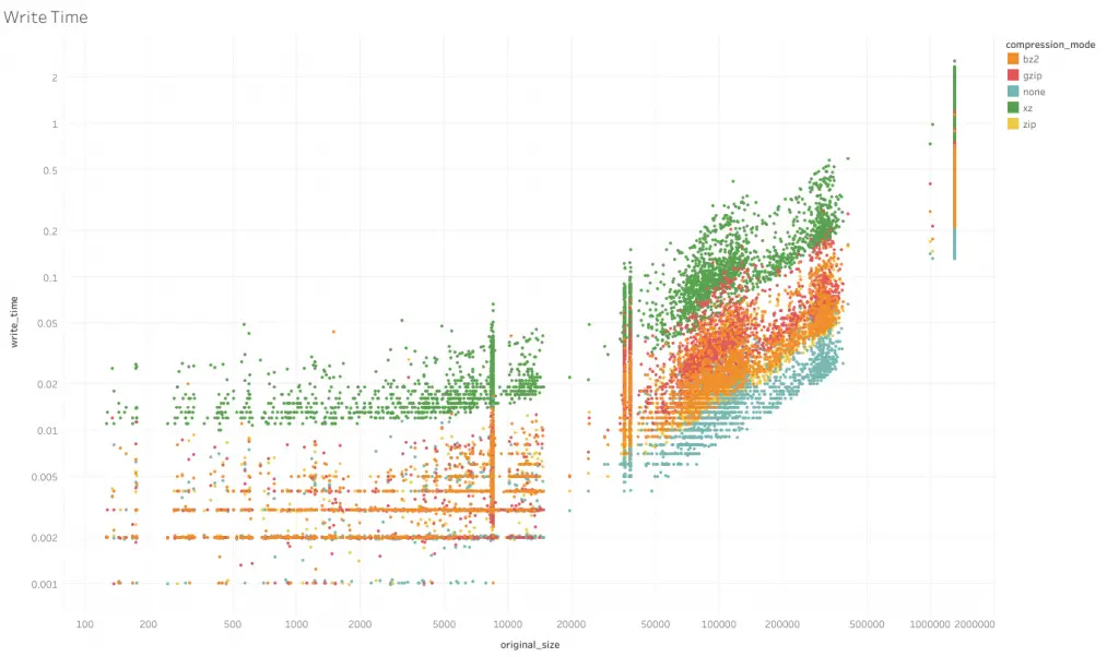
The horizontal axis of this chart is as before, size of uncompressed file in bytes on a log scale. The vertical axis is time required to complete the to_csv function, in seconds, also on a log scale.
Generally, formats that compress more take more time to write, as expected. Having no compression writes the fastest, followed by zip. xz writes the slowest. Between bz2 and gzip, this relationship appears not to hold. While earlier we saw bz2 compressing better than gzip, bz2 appears to take less time to write than gzip.
As for the shape of the graph, the trends are similar across formats. At smaller sizes time taken is almost the same regardless of size, possibly due to overheads. At larger file sizes, the log of time taken grows linearly with the log of the uncompressed file size.
Upon closer inspection (not in this graph), the trajectories of write time to file size differ even for the same format, depending of the content mix
Comparison of Read Speed
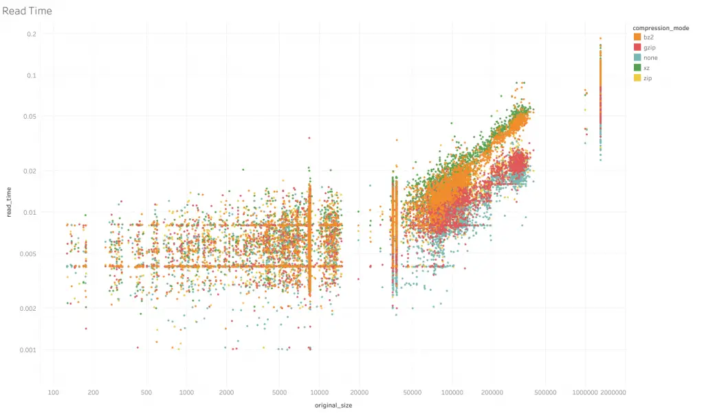
The axes are the same as for the write speed graph, except now the metric is for time required to complete read_csv.
Read speeds comparison across compression formats appear to be more in line with the compression rates. None has the fastest read times, followed by zip, gzip, bz2 and finally xz, which also has the highest compression rates.
Comparison of Contents
Obviously this is an important consideration. I’d assume file contents to be the same compressed, but thought I’d check just to be sure. For this I had only compared between the uncompressed version and the xz version. Strings looked fine. However with floats, the values differ at high precisions. Rounding them to approximately 10 decimal places matched the contents. If your use case requires higher than that level of precision, compressing data may present a concern. 10 was more than sufficient for my use case so I felt confident to proceed.
Conclusion
Given that my objective was to reduce storage costs, and the traffic-speed-bands dataset was by far the largest sized dataset, I adopted the xz compression mode for the project. xz performed the best for that dataset, and I was not too concerned with the additional read and write times. Overall capacity requirements came down about 90% after implementation of xz compression. For more details about the project, check out the Github repository here, and for the chart, on Tableau here.